Table of Contents
Preface
When you hear the term Fast Fourier Transform (FFT), you may immediately associate it with speed, signals, and fast computations. But what exactly is FFT, and how does it relate to the Discrete Fourier Transform (DFT)? This post dives into the core of these concepts, connecting the math behind them and highlighting why FFT revolutionized the way we compute frequency spectra.
🔍 What is the Fourier Transform?
The Fourier Transform is a powerful mathematical tool that transforms a signal from the time domain into the frequency domain. This means we can decompose the original signal to multiple basic sine/cosine waves, each with a specific frequency, and understand which frequencies are the main components of the original signal. This signals then helps to further downstream tasks, e.g.,
- Reveal hidden patterns: converts time-domain data such as sound, vibration etc into frequency domain to see periodic components or dominant frequencies.
- Enable signal filtering and compression: we can remove noise, compress data, or isolate important components once entering into the frequency domain. E.g., noise cancelling or environment sound simulation of your headset.
- Power spectrum estimation: used to estimate the power of different frequency bands in a signal. This is usually helpful for speech relevant tasks (Text-to-speech or speech-to-text) where in some approaches model can learn from the power spectrum features.
For digital applications, we use the discrete version — the Discrete Fourier Transform (DFT) — because computers can only handle finite, sampled data. While the original Fourier Transform is defined for continuous signals over infinite time, real-world digital systems (like audio recorders or sensors) can only capture signals at discrete time intervals and store a limited number of values. The DFT is specifically designed to work with these sampled signals, making it the practical choice for digital signal processing..
Note
👉 The following code and example are mainly referenced from the notebook Unit 9: Discrete Fourier Transform (DFT) from Prof. Meinard Müller in University of Erlangen-Nuremberg. I further added my own notes on top of it and did some exercises in my cloned notebook, which can be explored in Google Colab.
In this article, I try to keep only the necessary part for readers in order to quickly get to the point to explain the difference between DFT and FFT. Nonetheless, if you are interested in more details such as definition of inner product, rewriting a complex number in form of its polar representation, exercises etc., you can still find them in the notebook links provided above. Now let us dive in 😉
DFT: The Mathematical Foundation
We firstly define the notation of a signal. A signal in real-world that has been recorded and contains \(N\) data points is denoted as \(x \in \mathbb{R}^N \), so \(x[k], k=0,1,\dots,N-1 \) will be the k-th data point of the signal and its sign can be either positive or negative. A typical example would be a sine wave signal. Explanation to \(x[k] \in \mathbb{R}\) in the real world, can be, for example:
- In sound: negative values represent air pressure below ambient.
- In voltage: it means the signal is below the reference voltage.
- In displacement: it means movement in the opposite direction.
\(\textbf{Definition (DFT transform)}\) Given a signal \(x \in \mathbb{R}^N\), its discrete Fourier transform (DFT) is defined as a vector \(\hat{x} \in \mathbb{C}^N\) where:
$$
\begin{align*}
\hat{x}[k] = \sum_{n=0}^{N-1} x[n] \cdot \color{red}{e^{-\frac{i 2\pi k n}{N}}}
\equiv \sum_{n=0}^{N-1} x[n] \cdot \color{red}{\sigma_{N}^{kn}},~~~\forall~k=0,1,\dots,N-1
\tag{1} \label{eq:dft_vector}
\end{align*}
$$
Note:
- The vector \(\hat{x}\) can be interpreted as a frequency representation of the time-domain signal \(x\).
- Actually this DFT definition also applies to any signal \(x \in \mathbb{C}^N\), but we will stick with a real-valued signal that is closer to real-world problem and review one of its nice property: conjugate symmetry when \(x \in \mathbb{R}^N\).
- Intuitively, \(\hat{x}[k]\) means the inner product (or a similarity measure) between two signals: the original signal \(x\) and the basic sin/cos wave signal represented by \(e_k \in \mathbb{C}^N\) where \( e_k \equiv [1, \sigma_{k}^{N}, \sigma_{2k}^{N}, \cdots, \sigma_{(N-1)k}^{N}] \). Notice that its frequency is \(2\pi k /N \), which repeats itself after \(k=N\), and thus we only need to calculate for \(k=0,\dots,N-1\) and collect them to form \(\hat{x} \in \mathbb{C}^N\).
- This formula tells us how to compute each frequency component \(X[k]\). However, the computational cost is \(O(N^2)\), which can become very expensive for large signals.
\(\textbf{Example}\) Let us create an example signal \(x1\) of length \(N=64\) and duration 1 second that consists of three sine waves of different frequencies (\(1.9, 6.1, 20\)) and phases.
def generate_example_signal(dur=1, Fs=100):
    """Generate example signal

    Source: https://www.audiolabs-erlangen.de/resources/MIR/PCP/PCP_08_signal.html

    Args:
        dur: Duration (in seconds) of signal (Default value = 1)
        Fs: Sampling rate (in samples per second) (Default value = 100)

    Returns:
        x: Signal
        t: Time axis (in seconds)
    """
    N = int(Fs * dur)
    t = np.arange(N) / Fs
    # superimpose 3 different sine waves with different amplitudes
    x = 1 * np.sin(2 * np.pi * (1.9 * t - 0.3))
    x += 0.5 * np.sin(2 * np.pi * (6.1 * t - 0.1))
    x += 0.1 * np.sin(2 * np.pi * (20 * t - 0.2))
    return x, t

Fs = 64  # sampling rate in number of observations per second
dur = 1  # duration in seconds of a signal
x, t = generate_example_signal(Fs=Fs, dur=dur)We can then calculate its Discrete Fourier Transform (DFT) vector \( \hat{x} \) based on the previous definition. Since each element of \( \hat{x} \) is a complex number, we plot the real part and imaginary part separately in the following for each element \(k\). As mentioned before since \(\hat{x}[k]\) is a inner product measuring the similarity between \(x\) and \(\bar{e_k}\), we also show its absolute value (so as to ignore the similarity direction but only care about how strong the similarity is):
(Click to expand) Code to plot original signal \(x\) and its DFT transformed signal \(\hat{x}\) at various \(k\).
def plot_signal_e_k(ax, x, k, show_e=True, show_opt=False):
    """Plot signal and k-th DFT sinusoid

    Notebook: https://www.audiolabs-erlangen.de/resources/MIR/PCP/PCP_09_dft.html

    Args:
        ax: Axis handle
        x: Signal
        k: Index of DFT
        show_e: Shows cosine and sine (Default value = True)
        show_opt: Shows cosine with optimal phase (Default value = False)
    """
    N = len(x)
    time_index = np.arange(N)
    ax.plot(time_index, x, 'k', marker='.', markersize='10', linewidth=2.0, label='$x$')
    plt.xlabel('Time (samples)')
    e_k = np.exp(2 * np.pi * 1j * k * time_index / N)
    x_k = np.real(e_k)
    s_k = np.imag(e_k)
    X_k = np.vdot(e_k, x)

    plt.title(r'k = %d: Re($\hat{X}(k)$) = %0.2f, Im($\hat{X}(k)$) = %0.2f, $|\hat{X}(k)|$=%0.2f' %
              (k, X_k.real, X_k.imag, np.abs(X_k)))
    if show_e is True:
        ax.plot(time_index, x_k, 'r', marker='.', markersize='5',
                 linewidth=1.0, linestyle=':', label='$\mathrm{Re}(\overline{\mathbf{u}}_k)$')
        ax.plot(time_index, s_k, 'b', marker='.', markersize='5',
                 linewidth=1.0, linestyle=':', label='$\mathrm{Im}(\overline{\mathbf{u}}_k)$')
    if show_opt is True:
        phase_k = - np.angle(X_k) / (2 * np.pi)
        cos_k_opt = np.cos(2 * np.pi * (k * time_index / N - phase_k))
        # d_k = np.sum(x * cos_k_opt)
        ax.plot(time_index, cos_k_opt, 'g', marker='.', markersize='5',
                 linewidth=1.0, linestyle=':', label='$\cos_{k, opt}$')
    plt.grid()
    plt.legend(loc='lower right')


N = 64
x, t = generate_example_signal(Fs=N, dur=1)

plt.figure(figsize=(8, 15))
for k in range(0, 8):
    ax = plt.subplot(8, 1, k+1)
    plot_signal_e_k(ax, x, k=k)

plt.tight_layout()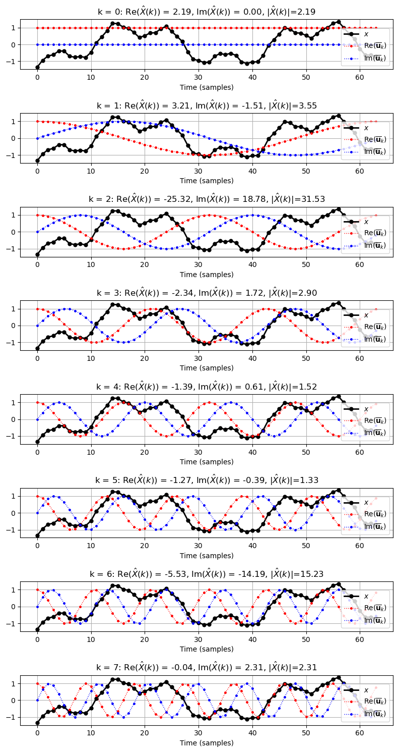
As shown in the above figure, the similarities are strong when \(k=2, 6\). This is no surprise since their corresponding frequencies are \(f_{k=2} = 2; f_{k=6} = 6\), which are very close to two of the three original sine waves frequencies \(1.9\) and \(6.1\).
In real world, of course we don’t know how the original signal \(x\) was made of. But through this example, we know that DFT helps us to extract important sine/cos waves of a given signal and thus can approximate and decompose the original signal into these critical components.
DFT in Matrix Form
We can express the DFT more compactly using matrix multiplication.
Recall that DFT of a signal \(x \in \mathbb{R}^N\) is defined as in \(\eqref{eq:dft_vector}\).
Then we can define a DFT matrix \(\mathrm{F}_N \in \mathbb{C}^{N \times N}\) as:
$$
\mathrm{F}_N = \begin{pmatrix}
1 & 1 & 1 & \dots & 1 \\
1 & \sigma_N & \sigma_N^2 & \dots & \sigma_N^{N-1} \\
1 & \sigma_N^2 & \sigma_N^4 & \dots & \sigma_N^{2(N-1)} \\
\vdots & \vdots & \vdots & \ddots & \vdots \\
1 & \sigma_N^{N-1} & \sigma_N^{2(N-1)} & \dots & \sigma_N^{(N-1)(N-1)} \\
\end{pmatrix}
_{N\times N}
\tag{2} \label{matrix:dft}
$$
Note:
- the \(k\)-th row of \(\mathrm{F}_N\) corresponds to the vector \(e_k \in \mathbb{C}^N\) mentioned previously, i.e., \(e_k = [1, \sigma_{N}^{k}, \sigma_{N}^{2k}, \cdots, \sigma_{N}^{(N-1)k}] \).
- The transformed DFT signal \(
\hat{x} = \begin{pmatrix}
\hat{x}_0 \\
\hat{x}_1 \\
\vdots \\
\hat{x}_{N-1} \\
\end{pmatrix}_{N \times 1}
= \begin{pmatrix}
e_0 \\
e_1 \\
\vdots \\
e_{N-1} \\
\end{pmatrix}_{N \times N}
\cdot \begin{pmatrix}
x_0 \\
x_1 \\
\vdots \\
x_{N-1} \\
\end{pmatrix}_{N \times 1}
= \mathrm{F}_N \cdot \begin{pmatrix}
x_0 \\
x_1 \\
\vdots \\
x_{N-1} \\
\end{pmatrix}
= \mathrm{F}_N \cdot x
\)
Below is the sample code to generate a DFT matrix and use it to transform a signal:
def generate_matrix_dft(K, N):
    """Generate a DFT (discete Fourier transfrom) matrix

    Notebook: https://www.audiolabs-erlangen.de/resources/MIR/PCP/PCP_09_dft.html

    Args:
        K: Number of frequency bins
        N: Number of samples

    Returns:
        dft: The DFT matrix
    """
    dft = np.zeros((K, N), dtype=np.complex128)
    time_index = np.arange(N)
    for k in range(K):
        dft[k, :] = np.exp(-2j * np.pi * k * time_index / N)
    return dft

def dft(x):
    """Compute the discete Fourier transfrom (DFT)

    Notebook: https://www.audiolabs-erlangen.de/resources/MIR/PCP/PCP_09_dft.html

    Args:
        x: Signal of shape N x 1 to be transformed

    Returns:
        X: Fourier transform of x with shape N x 1
    """
    x = x.astype(np.complex128)
    N = len(x)
    dft_mat = generate_matrix_dft(N, N)
    return np.dot(dft_mat, x)

N = 64
x, t = generate_example_signal(Fs=N, dur=1)
X_hat = dft(x)
This gives us a clean, linear-algebraic view on how we can apply a matrix on a given signal to obtain its discrete Fourier transform. However, the matrix computation \(\mathrm{F}_N \cdot x \) is expensive as it involves \(N \times N \) dense matrix with a \(N \times 1\) vector which results in \(\mathcal{O}(N^2)\) compute operations. This is where Fast Fourier Transform (FFT) kicks in and can help us speed up the matrix computation by observing and saving the repeated operations in the computation.
DFT Conjugate Symmetry
One of the nice property that DFT has is Conjugate symmetry whenever the signal \(x\) is real-valued. Let us look at the theorem.
\(\textbf{Theorem [Conjugate Symmetry]}\) Let \(x \in \mathbb{R}^N\). Then its DFT transform \(\hat{x}\) has the property:
$$
\hat{x}[m] = \overline{\hat{x}[N-m]}~~~\forall~m=0,\dots,N-1
$$
Proof can be found in 6.3. Conjugate Symmetry of Digital Signals Theory. Intuition behind the theorem is that the DFT vector has a symmetric structure where the real part are of the same values for each pair \((m, N-m)\) and the imaginary part are opposite. This means that we can calculate the DFT more efficiently and actually we even don’t need to calculate the whole spectral of frequencies from \(0\) to \(N-1\) to find critical frequencies and use them to approximate the real-valued signal \(x\).
Let us look at one example by using the same signal \(x \in \mathbb{R}^{64}\) generated previously.
If we collect all absolute values of each DFT element \(\{|\hat{x}_k|\}_{k=0}^{N-1}\), we will see that the plot \(|\hat{x}|\) generated by the following code is symmetric.
def plot_signal_dft(t, x, X_hat, ax_sec=False, ax_Hz=False, freq_half=False, figsize=(10, 2)):
    """Plotting function for signals and its magnitude DFT

    Notebook: https://www.audiolabs-erlangen.de/resources/MIR/PCP/PCP_09_dft.html

    Args:
        t: Time axis (given in seconds) of length N
        x: Signal of same length as `t`.
        X_hat: DFT of x of shape `len(x) x len(x)`.
        ax_sec: Plots time axis in seconds (Default value = False)
        ax_Hz: Plots frequency axis in Hertz (Default value = False)
        freq_half: Plots only low half of frequency coefficients (Default value = False)
        figsize: Size of figure (Default value = (10, 2))
    """
    N = len(x)
    K = N
    if freq_half is True:
        K = N // 2
        X_hat = X_hat[:K]

    plt.figure(figsize=figsize)
    ax = plt.subplot(1, 2, 1)
    ax.set_title('$x$ with $N=%d$' % N)
    if ax_sec is True:
        x_axis = t
        ax.set_xlabel('Time (seconds)')
    else:
        x_axis = range(len(x))
        ax.set_xlabel('Time (samples)')
    ax.plot(x_axis, x, 'k', marker='.', markersize='3', linewidth=0.5)
    ax.grid()

    ax = plt.subplot(1, 2, 2)
    ax.set_title('$|\hat{X}|$')
    if ax_Hz is True:
        Fs = 1 / (t[1] - t[0])
        x_axis = Fs * np.arange(K) / N
        ax.set_xlabel('Frequency (Hz)')
    else:
        x_axis = range(len(X_hat))
        ax.set_xlabel('Frequency (index)')
    ax.plot(np.abs(X_hat), 'k', marker='.', markersize='3', linewidth=0.5)
    ax.grid()
    plt.tight_layout()
    plt.show()

N = 64
x, t = generate_example_signal(Fs=N, dur=1)
X_hat = dft(x)

plot_signal_dft(t, x, X_hat)
plot_signal_dft(t, x, X_hat, ax_sec=True, ax_Hz=True)
plot_signal_dft(t, x, X_hat, ax_sec=True, ax_Hz=True, freq_half=True)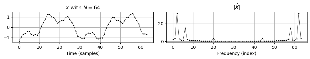
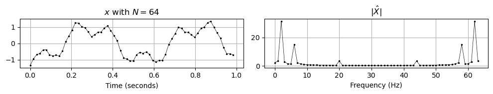
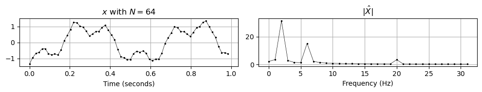
This symmetry is again due to the theorem conjugate symmetry where our input signal is real-valued. The plot also helps us identify at which frequency is the sin/cos wave has high similarity with \(x\) and thus can select that frequency as one of the components to compose \(x\). Furthermore, we don’t need to select the other half critical frequencies as they are the same as the first half of the critical frequencies due to symmetry. Bearing this observation in mind, FFT actually leverages the similar idea to speed up Fourier transform calculation by reusing the repeated calculations or patterns.
⚡Enter the FFT: Fast Fourier Transform
The Fast Fourier Transform (FFT) is not a new transform — it’s just an efficient algorithm to compute the DFT.
The key idea: reuse overlapping computations and exploit symmetries in the complex exponentials.
Properties of unit root
Before going to details, let us check \(\sigma_{N}^{kn}\)’s properties.
Recall that \(\sigma_{N} = e^{-i 2 \pi / N} = \cos(2\pi /N) – i \sin(2 \pi / N)\), then the following holds true:
- periodicity: \(\sigma_N\) has periodicity of \(N\), i.e., \(\sigma_{N}^{k+N} = \sigma_{N}^{k} \label{sigma:periodicity} \tag{3.1} \)
- symmetry: \(\sigma_{N}^{k+\frac{N}{2}} = – \sigma_{N}^{k} \label{sigma:symmetry} \tag{3.2}\)
- if \(m\) divides \(N\), then \(\sigma_{N}^{mkN} = \sigma_{N/m}^{kn} \label{sigma:division} \tag{3.3}\)
Intuition behind the periodicity is that, by Euler’s identity \(e^{i \pi} = -1\), we know that \(e^{i 2\pi} = 1\), hence \(\sigma_{N}^{N} = (\sigma_{N})^{N} = 1\), which proves the periodicity. And the symmetry property is also intuitive in that going through half-a-circle should be exactly at the opposite direction of the original value. Readers can easily prove these properties by replacing them with exponential form.
These properties are keys to reusing the similar computation patterns and will be used in the next section for Cooley-Tuckey Theorem.
Cooley-Tuckey Theorem
The FFT algorithm was originally found by Gauss in ca. 1805 and re-discovered by Cooley and Tukey in 1965. The algorithm leverages the properties mentioned previously to recursively break down the DFT matrix \(\mathrm{F}_N\) of size \(N\) into two DFTs of size \(\frac{N}{2}\) each, dramatically reducing computation.
Notice that the algorithm assumes the input length \(N\) is a power of 2 (radix-2). When it is not the case, the simplest way would be to pad the input sequence with zeros until its length is the next power of two. Nonetheless, there are actually other variants to deal with the situation, for more details please refer to Wiki Cooley-Tuckey Theorem Variations.
\(\textbf{Theorem (Cooley-Tuckey Algorithm)}\)
Formally,
$$
\begin{align}
\hat{x}_{N \times 1}
= \begin{pmatrix}
\hat{x}_0 \\
\hat{x}_1 \\
\vdots \\
\hat{x}_{N-1} \\
\end{pmatrix}
&=
F_N \cdot x_{N \times 1} \\
&=
\begin{bmatrix}
I_{\frac{N}{2}} & D_{\frac{N}{2}} \\
I_{\frac{N}{2}} & -D_{\frac{N}{2}} \\
\end{bmatrix}_{N \times N}
\begin{bmatrix}
F_{\frac{N}{2}} & O \\
O & F_{\frac{N}{2}} \\
\end{bmatrix}_{N \times N}
\begin{bmatrix}
\begin{pmatrix}
x_{even} \\
\end{pmatrix} \\
\begin{pmatrix}
x_{odd} \\
\end{pmatrix} \\
\end{bmatrix}_{N \times 1} \\
\\
&\text{, where }
D_{\frac{N}{2}} =
\begin{bmatrix}
1 & 0 & 0 & \cdots & 0 \\
0 & \sigma_{\frac{N}{2}} & 0 & \cdots & 0 \\
0 & 0 & (\sigma_{\frac{N}{2}})^{2} & \cdots & 0 \\
\vdots & \vdots & \vdots & \ddots & \vdots \\
0 & 0 & 0 & \cdots & (\sigma_{\frac{N}{2}})^{\frac{N}{2}-1} \\
\end{bmatrix}_{\frac{N}{2} \times \frac{N}{2}}
\tag{4} \label{thm:ct_fft}
\end{align}
$$
(Click to expand) \(\textbf{Proof:}\)
For simplicity, and WLOG, we assume the input signal \(x\) has length of power of 2. Even if it’s not, we can pad the signal sequence to power of 2 length.
$$
\begin{align*}
\hat{x}_k
&\stackrel{\eqref{matrix:dft}}{=} (F_{N})_{row=k} \cdot x~(~:= F_{N}^{k} \cdot x) \\
&\stackrel{\eqref{eq:dft_vector}}{=} \sum_n \sigma_{N}^{kn} \cdot x_n \\
&= \sum_{n=2t} \sigma_{N}^{kn} \cdot x_n + \sum_{n=2t+1} \sigma_{N}^{kn} \cdot x_n~(\text{split into even and odd})\\
&\stackrel{\eqref{sigma:division}}{=} \sum_{t} \sigma_{\frac{N}{2}}^{kt} \cdot x_{2t} + \sigma_{N}^{k} \sum_{t} \sigma_{\frac{N}{2}}^{kt} \cdot x_{2t + 1} \\
&= F_{\frac{N}{2}}^{k} \cdot x_{even} + \sigma_{N}^{k} F_{\frac{N}{2}}^{k} \cdot x_{odd}
\end{align*}
$$
where \(F_{\frac{N}{2}}^{k}\) is the Fourier transform of row \(k\) (freq \(k\)) with half periodicity \(\frac{N}{2}\) that is applied on the input signals \(\{x_n\}_{n=odd}\), \(\{x_n\}_{n=even}\) respectively, \(x_{even}\) and \(x_{odd}\) are vectors of size \(\frac{N}{2}\) collecting even and odd indices respectively. Similarly, one also obtains the formula for \(\hat{x}_{k + \frac{N}{2}}\) based on the unity root property describe above:
$$
\begin{equation}
\hat{x}_{k + \frac{N}{2}} = F_{\frac{N}{2}}^{k} \cdot x_{even} – \sigma_{N}^{k} F_{\frac{N}{2}}^{k} \cdot x_{odd}
\end{equation}
$$
From the above equations, it is not hard to see its recursive nature, and we can put them in the matrix form as well:
Define \(F_N\) as \(\{F_N^{k}\}_{k=0}^{N-1}\) stacked row-wisely, and define \(D_{\frac{N}{2}}\) as described in \(\eqref{thm:ct_fft}\). Then we can apply the above two formulas to the upper part and lower part of \(\hat{x}\) respectively:
$$
\begin{equation}
\hat{x}_{N \times 1}
=
\begin{pmatrix}
\hat{x}_0 \\
\hat{x}_1 \\
\vdots \\
\hat{x}_{\frac{N}{2}-1} \\
\hdashline
\hat{x}_{0 + \frac{N}{2}} \\
\hat{x}_{1 + \frac{N}{2}} \\
\vdots \\
\hat{x}_{\frac{N}{2} -1 + \frac{N}{2}} \\
\end{pmatrix}
=
\begin{pmatrix}
F_{\frac{N}{2}} \cdot x_{even} + D_{\frac{N}{2}} \cdot F_{\frac{N}{2}} \cdot x_{odd} \\
F_{\frac{N}{2}} \cdot x_{even} – D_{\frac{N}{2}} \cdot F_{\frac{N}{2}} \cdot x_{odd} \\
\end{pmatrix}
=
\begin{bmatrix}
I_{\frac{N}{2}} & D_{\frac{N}{2}} \\
I_{\frac{N}{2}} & -D_{\frac{N}{2}} \\
\end{bmatrix}_{N \times N}
\begin{bmatrix}
F_{\frac{N}{2}} & O \\
O & F_{\frac{N}{2}} \\
\end{bmatrix}_{N \times N}
\begin{bmatrix}
\begin{pmatrix}
x_{even} \\
\end{pmatrix} \\
\begin{pmatrix}
x_{odd} \\
\end{pmatrix} \\
\end{bmatrix}_{N \times 1}
\end{equation}
$$
which proves the theorem.
Example
Now let us see a concrete example on how Cooley-Tuckey Theorem works for a given signal and calculate its time complexity.
Assume \(x \in \mathbb{R}^8\). Since \(N=8\), we need to apply the theorem iteratively 3 times.
Apply the 1st time:
$$
\hat{x}_{8 \times 1}
=
\begin{pmatrix}
\hat{x}_0 \\
\hat{x}_1 \\
\vdots \\
\hat{x}_7 \\
\end{pmatrix}
= F_8 \cdot \begin{pmatrix}
x_0 \\
x_1 \\
\vdots \\
x_7 \\
\end{pmatrix}
=
\begin{bmatrix}
I_{4} & D_{4} \\
I_{4} & -D_{4} \\
\end{bmatrix}
\begin{bmatrix}
F_{4} & O \\
O & F_{4} \\
\end{bmatrix}
\begin{bmatrix}
\begin{pmatrix}
x_0 \\
x_2 \\
x_4 \\
x_6 \\
\end{pmatrix} \\
\begin{pmatrix}
x_1 \\
x_3 \\
x_5 \\
x_7 \\
\end{pmatrix} \\
\end{bmatrix}
$$
Notice that \(F_8 \cdot x\) (displayed in the middle above) will take \(64\) operations. This is the case when applying normal DFT. On the other hand, FFT already reduces some operations (displayed at the right hand side above) since the matrices are no longer dense.
Apply the 2nd time:
$$
\begin{cases}
F_{4} \cdot
\begin{pmatrix}
x_{0} \\
x_{2} \\
x_{4} \\
x_{6} \\
\end{pmatrix}
=
\begin{bmatrix}
I_{2} & D_{2} \\
I_{2} & -D_{2} \\
\end{bmatrix}
\begin{bmatrix}
F_{2} & O \\
O & F_{2} \\
\end{bmatrix}
\begin{bmatrix}
\begin{pmatrix}
x_{0} \\
x_{4} \\
\end{pmatrix} \\
\begin{pmatrix}
x_{2} \\
x_{6} \\
\end{pmatrix} \\
\end{bmatrix} \\
F_{4} \cdot
\begin{pmatrix}
x_{1} \\
x_{3} \\
x_{5} \\
x_{7} \\
\end{pmatrix}
=
\begin{bmatrix}
I_{2} & D_{2} \\
I_{2} & -D_{2} \\
\end{bmatrix}
\begin{bmatrix}
F_{2} & O \\
O & F_{2} \\
\end{bmatrix}
\begin{bmatrix}
\begin{pmatrix}
x_{1} \\
x_{5} \\
\end{pmatrix} \\
\begin{pmatrix}
x_{3} \\
x_{7} \\
\end{pmatrix} \\
\end{bmatrix}
\end{cases}
$$
Apply the 3rd time:
$$
\begin{cases}
F_{2} \cdot
\begin{pmatrix}
x_{0} \\
x_{4} \\
\end{pmatrix}
=
\begin{bmatrix}
I_{1} & D_{1} \\
I_{1} & -D_{1} \\
\end{bmatrix}
\begin{bmatrix}
F_{1} & O \\
O & F_{1} \\
\end{bmatrix}
\begin{bmatrix}
\begin{pmatrix}
x_{0} \\
\end{pmatrix} \\
\begin{pmatrix}
x_{4} \\
\end{pmatrix} \\
\end{bmatrix} \\
F_{2} \cdot
\begin{pmatrix}
x_{2} \\
x_{6} \\
\end{pmatrix}
=
\begin{bmatrix}
I_{1} & D_{1} \\
I_{1} & -D_{1} \\
\end{bmatrix}
\begin{bmatrix}
F_{1} & O \\
O & F_{1} \\
\end{bmatrix}
\begin{bmatrix}
\begin{pmatrix}
x_{2} \\
\end{pmatrix} \\
\begin{pmatrix}
x_{6} \\
\end{pmatrix} \\
\end{bmatrix} \\
F_{2} \cdot
\begin{pmatrix}
x_{1} \\
x_{5} \\
\end{pmatrix}
=
\begin{bmatrix}
I_{1} & D_{1} \\
I_{1} & -D_{1} \\
\end{bmatrix}
\begin{bmatrix}
F_{1} & O \\
O & F_{1} \\
\end{bmatrix}
\begin{bmatrix}
\begin{pmatrix}
x_{1} \\
\end{pmatrix} \\
\begin{pmatrix}
x_{5} \\
\end{pmatrix} \\
\end{bmatrix} \\
F_{2} \cdot
\begin{pmatrix}
x_{3} \\
x_{7} \\
\end{pmatrix}
=
\begin{bmatrix}
I_{1} & D_{1} \\
I_{1} & -D_{1} \\
\end{bmatrix}
\begin{bmatrix}
F_{1} & O \\
O & F_{1} \\
\end{bmatrix}
\begin{bmatrix}
\begin{pmatrix}
x_{3} \\
\end{pmatrix} \\
\begin{pmatrix}
x_{7} \\
\end{pmatrix} \\
\end{bmatrix} \\
\end{cases}
$$
The total operations needed will be dominated by \(\mathcal{O}(Nlog_2 N)\). For more details on the time complexity analysis, please refer to 8.2.3.1. Time analysis of Digital Signals Theory.
✅ Summary
| Feature | DFT | FFT |
|---|---|---|
| Description | Definition of frequency transform | Efficient algorithm for DFT |
| Formula | Direct summation | Recursive divide-and-conquer |
| Time complexity | \(\mathcal{O}(N^2)\) | \(\mathcal{O}(Nlog_2 N)\) |
| Use case | Conceptual foundation | Practical computation |
Hope this post gave you a clear understanding of how DFT works, and how FFT makes it fast. If you’re dealing with signals or doing spectral analysis — you’re almost certainly benefiting from FFT behind the scenes. Please also leave comments and I am happy to have open discussions with you!